Distances on Markov Chains and their Differentiation
Tristan Brugère
Zhengchao Wan
Yusu Wang
The 35th International Conference on Algorithmic Learning Theory (2024)
1 Introduction
1.1 Introductions


1.2 Motivation: Learning on graphs
(labeled) Graphs are everywhere
- Chips (directed, labeled, multigraphs)
- Molecular structures
- Social networks
Discrete or continuous features
We want to
- Compute statistics on graph datasets;
- Make NNs that output graphs
1.3 Problem
\[\text{Loss}(G) = \text{\large\textbf{?}}\]
\[\text{Loss}(G) = d_{\text{graphs}}(G, G_{\text{target}})\]
\[d_{\text{graphs}} = \text{\large\textbf{?}}\]
And we want this loss to be differentiable (for gradient descent).
1.4 Comparing graphs is hard
- Independent of data representation / node ordering

No Polynomial algorithm for graph isomorphism
Graphs are combinatorial objects (how do we differentiate on the space of graphs?)
1.5 SOTA: FGW
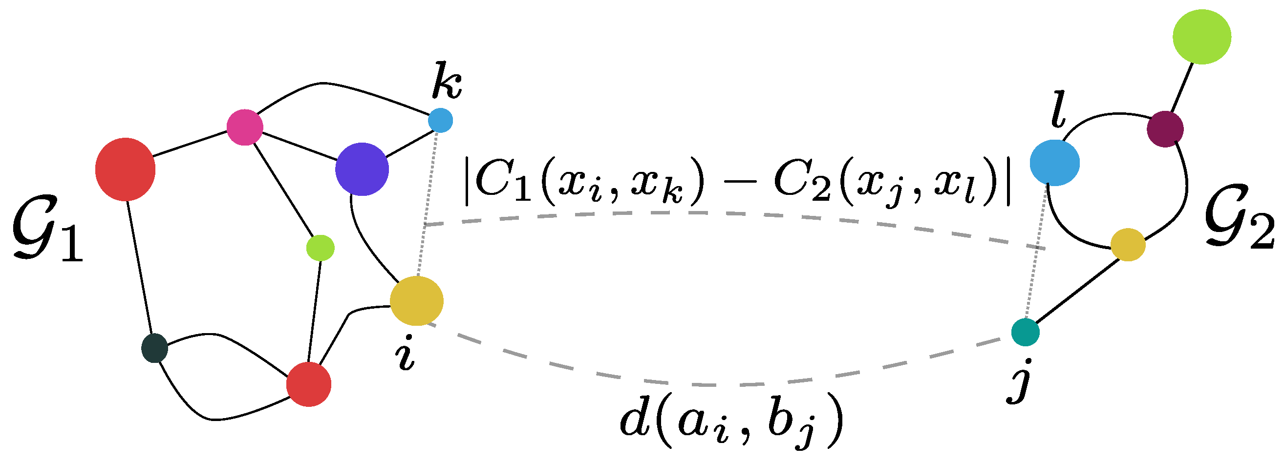
Fused Gromov Wassertein distance (FGW):
See graphs as metric spaces
Compute a matching of nodes minimizing:
- Distance between node features;
- Distortion of the metric structure
1.6 Challenges with FGW:
- No differentiation
- (but can be minimized by a heuristic procedure)
- Computation is heuristic
- (no guarantee of convergence)
- Intuition does not apply to directed graphs
1.7 Preliminaries:

Markov chain
- Memoryless random walk
- On a space of “states”
- Next state distribution depends only on the current state
Optimal Transport (Wasserstein’s distance, Earth mover’s distance…)
- Compute a soft matching between pointsets
- minimize that cost
2 Our approach
2.1 From Graph to Markov Chain
\[\text{(labeled) Graph } \simeq \text{ (labeled) Markov Chain}\]
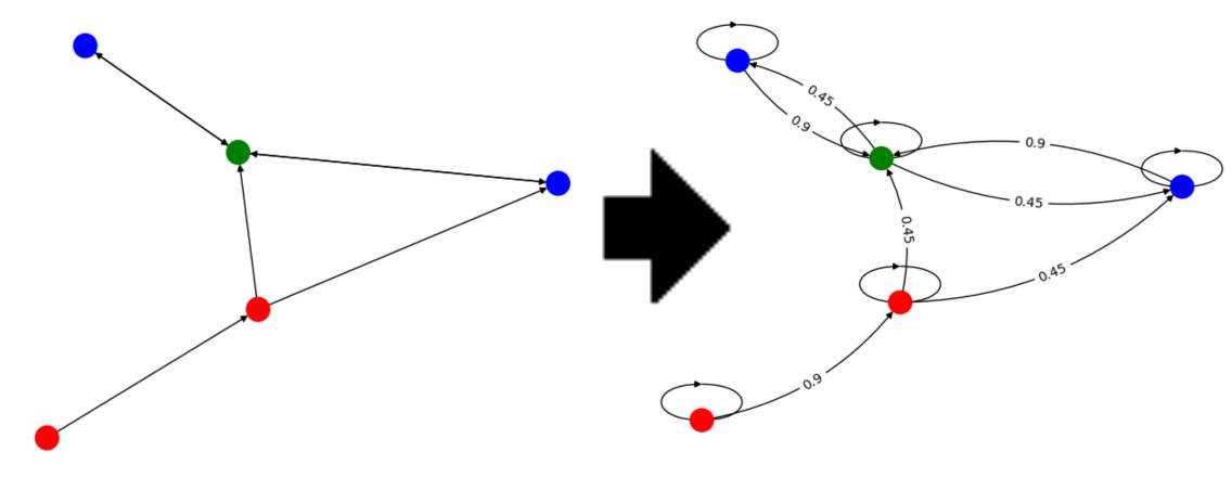
- Random walk gives a Continuous representation of the combinatiorial object
2.2 Optimal transport on Markov Chains
Regular
Markov
Pointset law \((p_X, p_X)\)
Markov Chains \((\mathcal{X}, \mathcal{Y})\)
\(C(X, Y)\) between points
\(C(X_i, Y_i)\) between states
Take \(p\) distribution over \(\N\) and \(T \sim p\) independent of \(X\) and \(Y\)
\[d_{OT}(p_X, p_Y; C) = \inf_{\substack{(X, Y) \text{ coupling} \\ X\sim p_X \\ Y\sim p_Y}} \E\, C(X,Y)\]
\[d_{???}(\mathcal{X}, \mathcal{Y}; C) = \inf_{\substack{(X_t, Y_t) {\color{#D462AD}\text{ Markovian coupling } }\\ X_t\sim \mathcal{X} \\ Y_t \sim \mathcal{Y}}} \E\, C(X_{\color{#D462AD} t},Y_{\color{#D462AD} t})\]
\[d_{\color{#6E963B}OTM}(\mathcal{X}, \mathcal{Y}; C) = \inf_{\substack{(X_t, Y_t) {\color{#D462AD}\text{ Markovian coupling } }\\ X_t\sim \mathcal{X} \\ Y_t \sim \mathcal{Y}}} \E\, C(X_{\color{#6E963B} T},Y_{\color{#6E963B} T})\]
2.3 Contributions: Theoretical Framework
Study of optimal transport method for Markov chains
Theoretical framework: Optimal transport Markov (OTM) distances.
- links previous Optimal transport-based methods on Markov chains.
- (Moulos 2021)
- (O’Connor et al. 2021)
- (Chen et al. 2022)
2.4 Contributions: DDWL-Distance
particular case of interest: \(\delta\)-discounted WL distances.
Differentiable
- In the label values and the Markov chain structure
- With some regularization
Computationally tractable
- converging iterative algorithm
Naturally adapted to directed graphs
Can work with non-stationary Markov chains
- adds stability over previous Markov-based methods
2.5 Intuition
Similar to the Weisfeiler-Lehman isomorphism test
Or to an MPNN
“Propagate” labels from neighbors to neighbors (random walk)
Determine “how different” the label distributions are
2.6 Formalization

2.7 Experiment: noisy circle barycenter
Compute by gradient descent: \[\text{Barycenter}(G_1, G_2, \dots, G_n) = \inf_{G} \sum d(G, G_i)^2\]
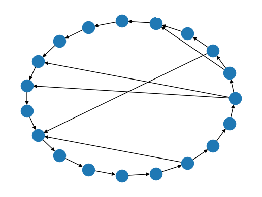
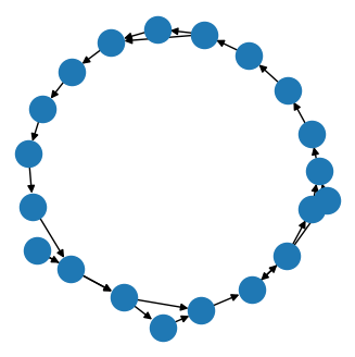
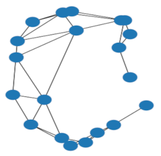
Example output of the barycenter experiment on circle graphs with Erdős–Rényi noise
2.8 Experiment: Synthetic data — noisy circle barycenter (II)
3 Conclusion
3.1 Current challenges and future work
Computationally expensive
Ongoing work on generative models
3.2 Thank you!
3.2.1 Code
$ pip install ot_markov_distances3.2.2 Contact
3.2.3 Acknowledgements
This work is partially supported by NSF under grants CCF-2112665, CCF-2217058, and CCF-2310411.


